Flow Simulation’s Thermal Analysis Capabilities

For thermal heat transfer analysis, choose SOLIDWORKS Flow Simulation over the Thermal solver in Simulation Professional, Part 3 of 3 Meshing

With the exception of very few scenarios, when considering a thermal analysis solver for SOLIDWORKS, you should choose to use Flow Simulation, which is a computational fluid dynamics (CFD) code. The most typical exceptions would be when: (1) there is no convective heat transfer mechanism in the problem that is being solved because likely the object(s) are in a vacuum and only transport heat through conduction and radiation; or (2) the thermal solution does not require a great deal of accuracy reflecting a physical test perhaps in the very early design stages when estimates are sufficient. The main 3 reasons why Flow Simulation is the better option will be outlined in a series of three parts.

As noted above, there are three modes of heat transfer: conduction, convection and radiation. I’ve made a long-form video explaining all of these modes in more detail, see link at the bottom, so I will only summarize them here in the series. Also the superior approach to meshing in Flow Simulation was browsed over in the video, in order to keep the video from getting any longer, but it is a very important aspect to this argument so it will be highlighted here in part 3.

3. Simulation Professional mesher works well only if there are no geometry interferences; Flow Simulation mesher is very tolerant of complex geometry even when there are interferences

The mesher in Simulation Professional is very different from the way meshing is done in Flow Simulation, and because of this the Simulation Professional mesher cannot handle common geometry issues, such as when two bodies are overlapping or interfere. It’s very common that designers take shortcuts when running CAD because it’s in a virtual environment where some items such as holes or other features will be added later in manufacturing to make it work. We have to face the fact that the way that CAD is used for manufacturing is different than what is needed for CAE. But analysis programs typically cannot tolerate shortcuts in CAD that lead to less than desirable geometry, for example, pins of board components that push through PCBs. Also on the other side of the spectrum, a designer could include every detail in the model from small external fillets for aesthetic purposes to threads on a fastener. Image 11 shows an example of typical CAD geometry of a pin that interferes with the PCB on which it is placed, and note that there are more than 100 counts of similar interferences in this assembly.

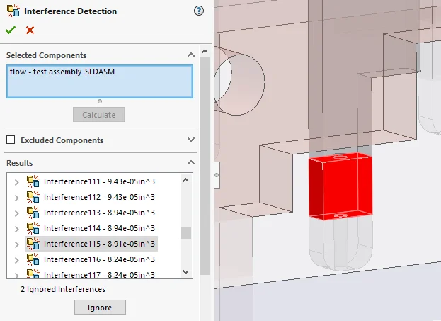
Image 11: Typical interference of a pin with a PCB.

Flow Simulation handles the problem of meshing interferences both with setting up material priorities and with a proprietary way that the computational cells are treated. When setting up a Flow Simulation project in the Wizard, where heat conduction in solids is included, a default solid material must be chosen; this ensures that all parts have at least a solid material defined. In the Flow Simulation feature tree, solid materials can be specified for all components that are not made of the default solid material or imported from the material defined inside the CAD model definitions. The newly defined material in the feature tree have a higher priority than the default material, but materials can manually be reordered. In Image 12, the Insulator material was manually moved below the default material into fifth position and the specific 4-signal 2-power (4s2p) PCB generated material has the lowest priority. What this means is that a material having a higher priority will be used where two bodies are overlapping, so that solves that one issue.

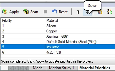
Image 12: Material Priorities dialog in Flow Simulation; the Insulator material was manually moved down to fifth position.

If you already read the first post in this series, you’ll recall an example regulator microchip problem where the different mesh schemes was briefly mentioned to be covered in part 3. Simulation Professional uses the finite element method (FEM), where the mesh elements need a defined connectivity between its nodes and an element has to be constrained within a single body, which would seem to be a standard requirement. This single body requirement does become a limitation when applied to real geometry, where the overall size to thickness (or aspect ratio) is quite large. Zooming into the bodies between the large microchip at top and the copper heat sink at bottom, in Image 13, shows there are two layers of material in between. The thinnest part is only 25 mm thick but is 21.2 mm in its longest edge resulting in an aspect ratio of 848. Mesh controls in Simulation Professional are able to capture this body after the default mesh settings failed to mesh this part, as seen in Image 14.

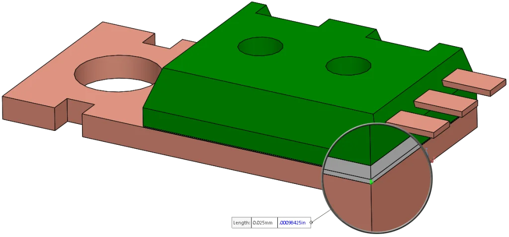
Image 13: Magnifying glass (hotkey: G) zoomed in measurement of the thermal paste layer shows a thickness of 25 mm (0.025 mm).

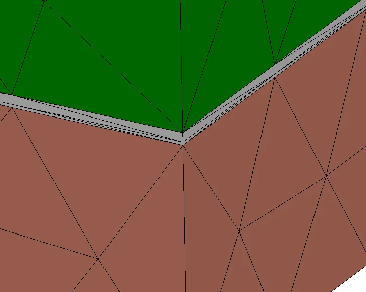
Image 14: Finished finite element mesh after mesh settings in Simulation Professional were employed.

In part 2, cells were introduced as the basic computational unit in the Finite Volume (FV) approach used by Flow Simulation. A basic premise of the cell is that calculated values are stored at the cell center, instead using nodes in the finite element method, so as a consequence of this for the FV method is that connectivity is irrelevant. Thus a finite volume mesh can have more than one cell that is sharing a face of its adjacent cell, although for other reasons related to solver specifics, Flow Simulation limits this difference to one level of difference. The FV mesh can notch down over many levels to reach the required sized to capture any complex geometry or flow field gradient as required, see Image 15 as an example using the lamp with reflector model from the second post. The final computational mesh shown comes from both initial local mesh refinement to capture the geometry and a single adaptive refinement (during the solution) to capture the velocity and temperature gradients in the rising lower density air. Level 0 in blue are known as the base “parent” cells, and levels 1 and higher are “daughter” cut cells.

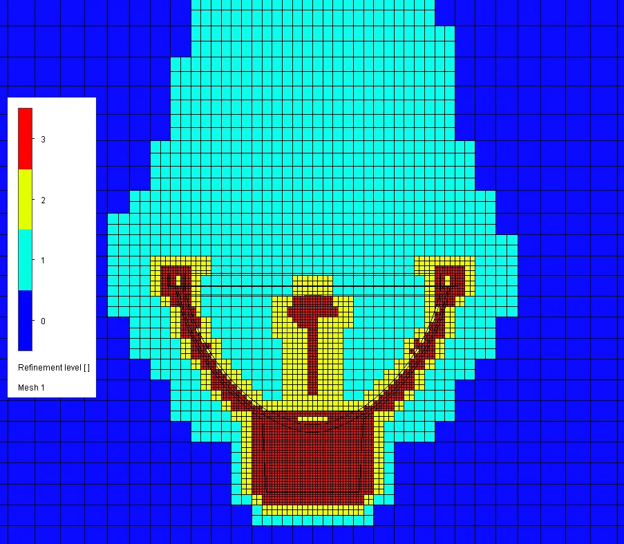
Image 15: Mesh refinement levels from the base “parent” level 0, cut one level down to capture rising air currents, finally to level 3 to capture the bulb and reflector geometries.

But underlying all of this is the most exciting and interesting bit about the cell technology proprietary to Flow Simulation, called SmartCells®, is that it breaks the paradigm of one cell to a single body, solid or fluid. A whitepaper (see link below) on the technology describes them as:

SmartCells are Cartesian based meshes that are typically 10 times smaller in size than traditional CFD meshes while providing the same level of flow field resolution and attaining high levels of simulation accuracy.

While the meshes are much coarser than is recommended for more accurate results, the following two images both exemplify the extent to which SmartCell technology can be useful for difficult geometry.

The regulator microchip in Image 16 shows that a single SmartCell is able to span 4 different solids with each having a different material property. Compare how this approach is much easier and more reliable than what had to be done for the finite element mesh in Image 14 earlier. This is an easier example, but for some models it might not be practical to create a mesh for Simulation Professional, without the user having to put in much more time and effort to the fix issues created by that process. I contend that software should be able to bend to the way the user wants to use the software, and not have the user bend to the conventions created by the method employed in the program.

If you are a keen observer, you would had noticed that the temperature change accurately reflects the difference in thermal resistance based on a material’s conductivity. Also note in the mesh another instance of multiple body/material changes in the image at the top, where the connector protrudes from the chip; even if it was the case that the chip interfered with the copper connector, the material priority discussed earlier would handle the change in resistance.

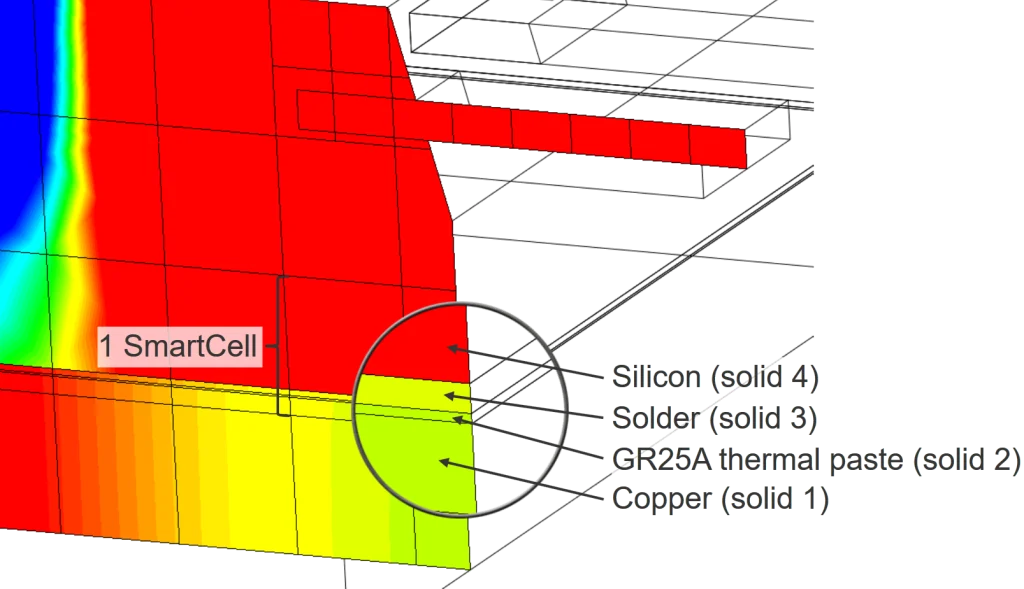
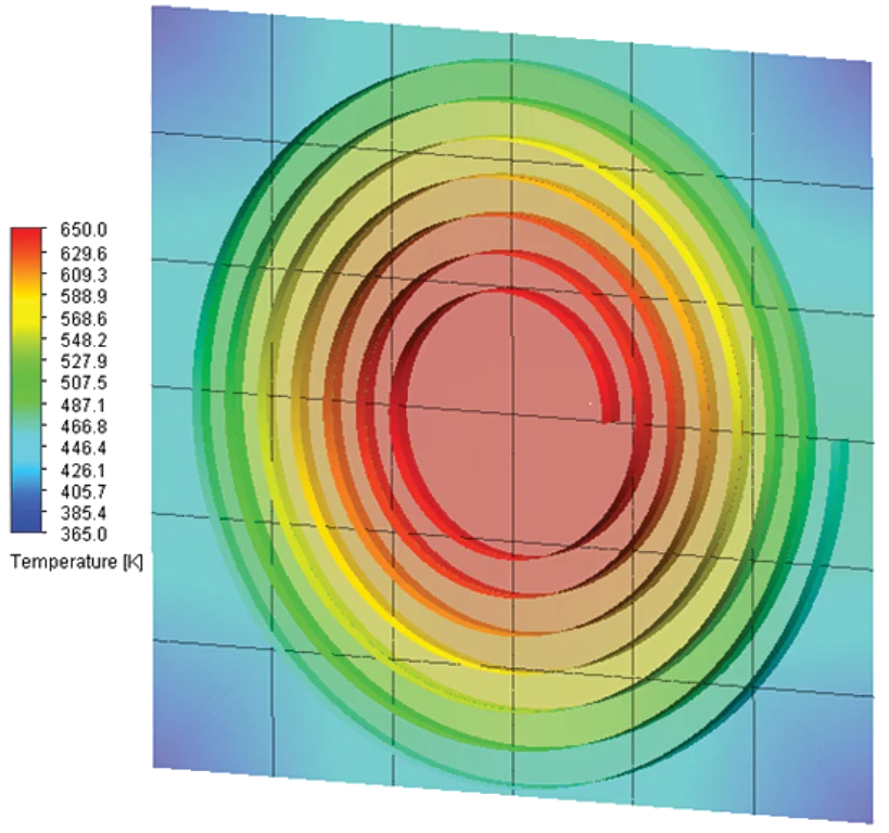
Image 16: A single SmartCell in the regulator microchip model spans 4 different solids each having a different material; the temperature legend values were narrowed to better highlight zoomed features.

While on the topic of resistance, Flow Simulation also supports Joule (or Ohmic) heating, where you can apply a direct current or voltage potential to a material that has an electrical resistance to determine the amount of heat power that it dissipates. The wound coil in Image 17 shows an example of this Joule heating while simultaneously demonstrating how a single SmartCell has multiple fluid-solid boundary crossings.

Image 17: SmartCells span across multiple solid-ﬂuid boundaries in simulating wound coil heated by an electric current.

I will conclude this series of blog posts on this topic with a single image that encompasses all that I had hoped to express throughout in words: a full fidelity geometry; the irregular distribution of temperatures is emblematic of the realistic results having used all modes of heat transfer; and the mesh is both localized to the important geometry features and adaptively refined to the solution. In more simple terms, I simply recommend Flow Simulation by saying, “It just gets the job done,” without me having to worry whether it’s going to work or not.

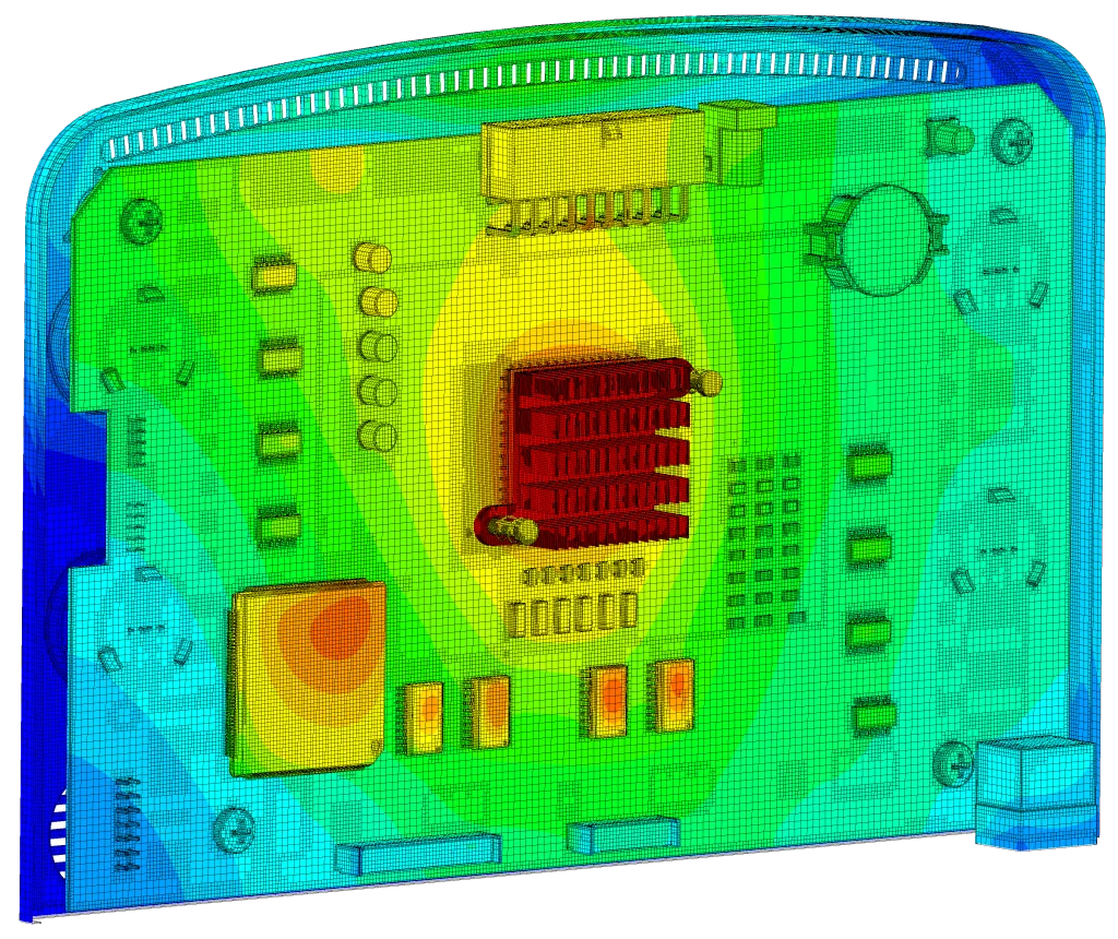
Image 18: Surface plot of temperature (with the final adaptive refinement mesh) for a conjugate heat transfer solution of a smart refrigerator panel done in SOLIDWORKS Flow Simulation.

Link to the whitepaper “SmartCells® Enabling Fast & Accurate CFD” click here.

Did you enjoy this series? Be sure to check back on the SOLIDWORKS Tech Blog to learn more about Flow Simulation’s Thermal Analysis Capabilities! Incase you missed it, take a look back on Part 1 and Part 2.

Bio
Twitter
LinkedIn
Latest Posts

Joe Galliera

Senior Simulation Technical Manager , East area at DS SOLIDWORKS

Joe Galliera has been with SOLIDWORKS since 2002. Previously he worked in the aerospace industry primarily focusing on computational methods. He geeks out on computational fluid dynamics (CFD) and nonlinear analysis.