
How many different ways are there to solve a Simulation problem? There are probably many more ways than you think, so you may be asking yourself: “How can I be sure that I have the ‘right’ answer?”
First off, while one could come up with a myriad of different answers for the same problem, there are no “right” answers, just one that is generally agreed upon. What I mean by this is that the program gives the user a very specific answer to a question that it is asked. Sort of like a black box: a question goes in, and an answer is spit back out. The problem that the user faces is whether the proper question is asked.
A very good piece of advice that I learned some time ago from a colleague that I will share with you is that every input (into an FEA program) is an assumption.
- Starting with the geometry: Is this the exact geometry that will be physically made? No, the CAD model is an idealization of the real thing. And then you discretize the geometry with a mesh, further removing it from reality.
- The material properties will most definitely be different. Are there any microscopic imperfections in the finished part that may cause it to fail sooner?
- Will the forces and restraints ever change location, magnitude and direction? And what about the value, where did that come from, and are you certain that it won’t be different?
- Can you predict all the different ways that the design will be used in the field? Have you ever seen wrench used as a hammer?
- Conducting a proper simulation requires the user to manage the assumptions.
Is it then even worth running a simulation? Yes. There is still a ton of valuable information that you can obtain from the results. To answer the question, is there a right answer: All answers are wrong, and only some are useful. I found an interesting post on the SOLIDWORKS Forums some years ago that I will use an as example problem to demonstrate how there are several ways of solving the same problem. The reason I like this example is because the original poster provided a 2D image of the model and an actual photo of the buckle part.
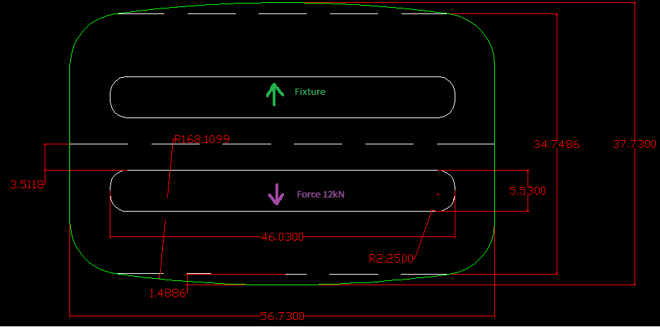
Image 1: 2D drawing of the example model with dimensions given in millimeters.
In the drawing, a force of 12 kN is indicated pushing down with a fixture holding it up. The dimensions are detailed in millimeters and the poster stated that it is 3.25mm thick. A material is also provided, but I will explain shortly why this is really not immediately important. From the photo in Image 2 of the actual part, you can tell that it is made from a metal.
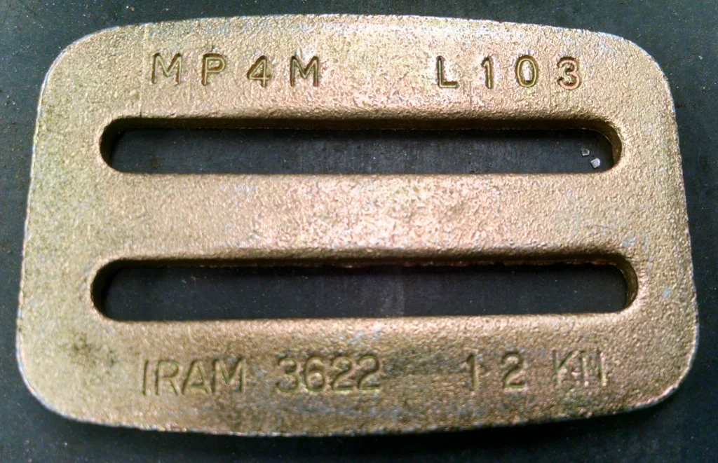
Image 2: Photograph of the actual physical part.
When I model up the part and run it exactly as stated, I get the following error message seen in Image 3, “No restraints are defined.” The reason is that the solver cannot come to a unique solution; any small difference can cause the forces to not exactly balance out in all directions. It’s NOT because I had not stated what the material is yet. When looking at stresses, the equation of load over geometric section does not include material properties. Yes, to run an FEA problem, you need to define a material, but don’t sweat it, just apply any material and you’ll get the same results. Don’t believe me, try it yourself. (Now if you are focusing on displacements then this is another thing.) Only after you know what the stresses are should you start to look for a material whose properties meets those requirements (and cost obviously, not everything can be made from Wishalloy.)
Doing what the error message suggests provides just enough for it to solve. This is one way, the first way in our case, to solve the problem.
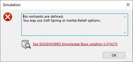
Image 3: Error message that there are not sufficient restraints to solve the problem as exactly stated.
This is not what I would call a good solution though because clearly you can see in Image 4 that the displacements are off. I did not alter (by rotating) the image; this is the answer that was spit out. The deformations are automatically exaggerated by over 4 times, and this is done normally so that you can see what are typically very small displacements. The unknown quantities solved for in a static problem are displacements, so this is important. The stress distribution seems to make sense, so I can get some information from this result.
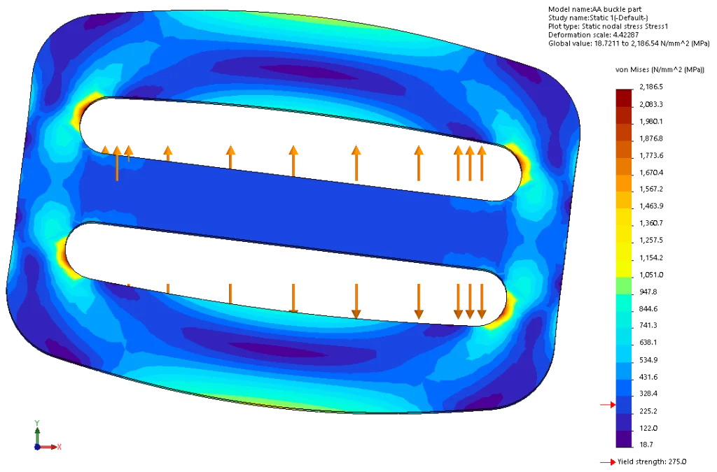
Image 4: Solution #1 set up as original problem statement. Opposing load vectors are shown vertically while the rotated deformation is scaled over 4 times.
One commenter suggested applying restraints at strategic points in order for the solver to run. For this example, I applied normal (perpendicular to the screen) and vertical restraints at two vertices towards the top of the part on either side; and at a single vertex on the bottom middle, another normal restraint and a horizontal restraint to prevent it from moving side-to-side but still allowing it to stretch vertically there. You can see the remnants of the three pinned restraints boxed in red in the Image 5 stress results below. This allows the model to run normally, but I would not suggest using this method universally. It can cause some very large stress risers for some solutions; think of the way a t-shirt hangs when it is pinned on a clothesline. The deformations are scaled by over 16 times.
Now another way to solve the problem is by knowing that the restraints will exert an equal and opposite reaction force, so the load applied vertically up could instead be defined as a vertical restraint. Actually, I took the liberty of switching out the “fixture” in the 2D drawing for a load because of this fact. It’s important to note that a restraint prevents the selected feature from moving at all, so this is why I initially dismissed it. For example, if I applied a vertical restraint at the face instead, it would be flat and would not take the rounded shape that is shown. So remember that restraints are definite (d = 0), and they do not exist in nature. Solution #3 is not shown here, but you can see the setup and results from the attached part file. (The part was saved in SOLIDWORKS 2019 SP3.0 and can be downloaded from this link: https://bit.ly/SimBlog625)
With a couple results, we can start to see some similarities. The maximum stresses are around the inside radii of the holes and are away from the loads and restraints. The only thing that changed from Solution #1 to #2 was adding the pinned restraints. The mesh is exactly the same, so the max and min values are the same. Most importantly the results appear to be symmetric. They look to be symmetric from top to bottom and right to left; it is also symmetric from front to back (not shown). If we check the geometry, material properties, loads and restraints, they are all symmetric in all three directions. Know that the definitive indicator whether a problem can be solved using symmetry is, and always will be, the results of the full model. This is most important for a nonlinear problem where the solution may yield non-symmetric results even if all other things (inputs as stated previously) are symmetric.
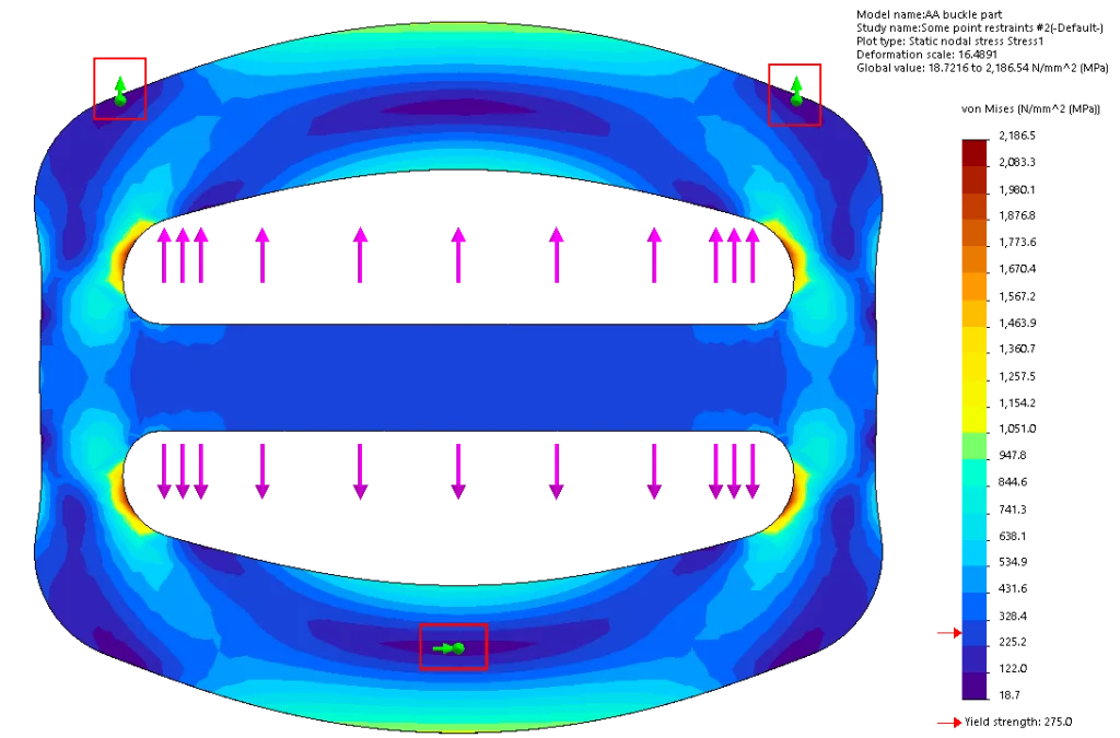
Image 5: Stress results from the Solution #2 showing remnants of the three pinned restraints boxed in red.
We can exploit the symmetric looking results to our advantage to really solve this problem most efficiently by solving just 1/8 of the model. You can use a SOLIDWORKS tool in the Evaluate tab called “Symmetry Check,” see Image 6, to automatically split the part along all planes of symmetry. Choose the body that you want to keep and select split to have the software make quick work of it. I made a new configuration from the new features (four planes and split) that the software automatically added for me.
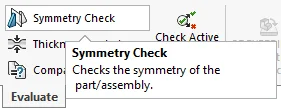
Image 6: Symmetry Check in the Evaluate tab of the Command Manager toolbar.
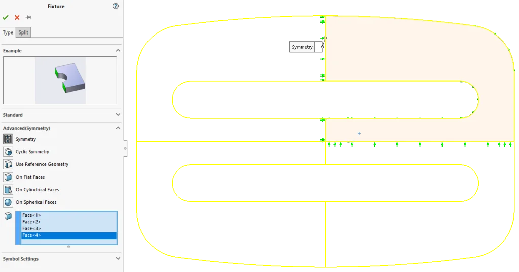
Image 7: Adding the Symmetry fixtures in the three coordinate directions, on four faces, reveals an outline of the full model where I can later show the mirrored results.
By applying the symmetry in the three coordinate directions, I have a fully restrained model. Because symmetry is a natural condition, they do not affect the results other than assuming that the results are symmetric. What I mean by symmetry being natural is that there is material on the other side of the boundary condition being simulated; the part cannot translate apart from or rotate out of plane (in two directions) of the material across those faces.
The results for the Solution #4 are shown below in Image 8. The load that I applied to the buckle face is only one-quarter of the full load value because only 1/4 of the original face still remains. The resultant stresses align well with the previous results that we have seen, with the maximum only changing by about 122 MPa over about 2310 MPa, or about 5.3%. No mesh convergence has been investigated yet, just running default settings, so the difference could be narrowed down. You can see the lines where the results are mirrored, and even though the front upper right portion is meshed and solved, you can view, animate and probe results anywhere as if it was a full model solved.
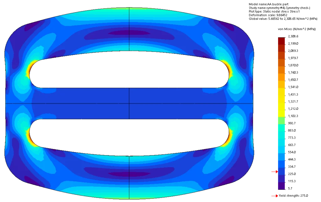
Image 8: Solution #4 where symmetry results are mirrored from solving only 1/8 of the full model in the front upper right section of the part.
Taking this another step further, I realize that results also appear to be as if it were simulated as a 2D problem. It looks like the results are the same through the thickness such that they appear to be extruded, although they are not. When I set up a new study, I can choose the “Use 2D Simplification” option for the Static study, see Image 9. There’s an additional step for the 2D simplification, after clicking the green OK check mark, where the type of 2D model is selected, see Image 10. The first type, Plane Stress, is the proper one to use here, because as the animation and description show, it is for a relatively thin geometry and where stresses do not vary normal to the section plane, as I had described above. I choose the Front plane as the Section place and define its depth, but this is only used for 3D visualization. A helpful preview of the Section plane that is extracted from the geometry is shown in the graphics window.
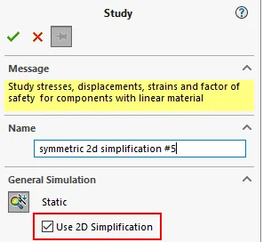
Image 9: Use 2D Simplification option for a Static study.
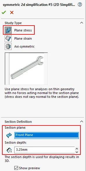
Image 10: Defining the Plane Stress 2D study type by defining the Section plane and depth.
I have to define the load value by considering the Section definition, where the original face for applying the load is now an edge characterizing the full width of the part, and is only half-symmetric side-to-side so I apply 1/2 of the load for this problem. I can define symmetry conditions on the other edges that were cut from the original full model and solve the problem. I get a very fast solution from the 2D simplified model, because there are much fewer elements to cover the model. The results, shown in Image 11, are practically identical to the previous result. The difference in maximum stress from the previous solution is less than 1 percent.
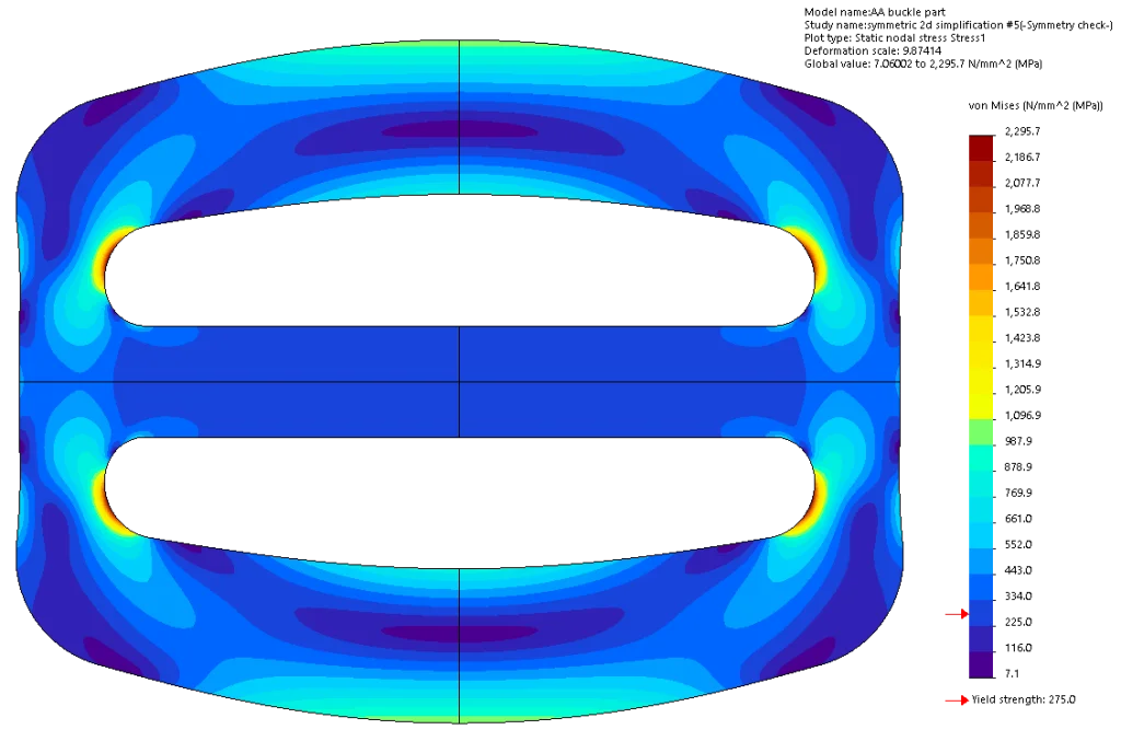
Image 11: Solution #5 using the 2D Simplification Plane Stress study type with quarter-symmetry conditions.
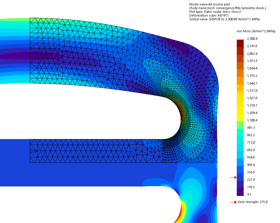
Because I’ve been able to pare this model down to just what’s needed, it runs in a matter of seconds, so to be complete with this model, I should run a mesh convergence study to check whether the mesh has an impact on the result. Global mesh setting is slide down all the way to fine setting, and a local mesh control is applied to the rounded cut. The results with the mesh overlaid on top are shown in Image 12, and maximum stress differs by only 0.226% from the previous solution. So we can finally say that the results of all 6 solutions general agree.

Image 12: Solution #6 from doing a mesh convergence study of the 2D Simplification Plane Stress model.
(The part was saved in SOLIDWORKS 2019 SP3.0 and can be downloaded from this link: https://bit.ly/SimBlog625)