Flow Simulation’s Thermal Analysis Capabilities

For thermal heat transfer analysis, choose SOLIDWORKS Flow Simulation over the Thermal solver in Simulation Professional, Part 2 of 3 Conjugate Heat Transfer

With the exception of very few scenarios, when considering a thermal analysis solver for SOLIDWORKS, you should choose to use Flow Simulation, which is a computational fluid dynamics (CFD) code. The most typical exceptions would be when: (1) there is no convective heat transfer mechanism in the problem that is being solved because likely the object(s) are in a vacuum and only transport heat through conduction and radiation; or (2) the thermal solution does not require a great deal of accuracy reflecting a physical test perhaps in the very early design stages when estimates are sufficient. The main 3 reasons why Flow Simulation is the better option will be outlined in a series of three parts.

As noted above, there are three modes of heat transfer: conduction, convection and radiation. I’ve made a long-form video explaining all of these modes in more detail, see link at the bottom, so I will only summarize them here in the series.

2. Flow Simulation is better suited to solving conjugate heat transfer problems.

Did you know that before the 1960’s, the process to solve conduction, convection and radiation was to handle them separately? As you might expect, this was not an accurate approach to solving the real physical process. In more recent years with the subsequent advancement of computational analysis, a new approach to combine the heat transfer processes together was taken, so a “conjugate” heat transfer problem is combining any of the two (or all three) modes to be solved concurrently.

Flow Simulation uses a Finite Volume (FV) method to solve the CFD equations, where three conservation methods (mass, momentum and energy) and the state equation are all maintained. In other words, pressure, temperature, velocity and the fluid properties are all tightly dependent on one another. The set of all these highly nonlinear coupled equations are iteratively solved for a given discretized geometry (or mesh) and boundary conditions (BC’s). It can take some time to solve a thermal CFD problem, perhaps a few minutes to a several hours depending on the complexity of the problem. But the good thing is that the user inputs can be as simple as setting the ambient temperature and pressure, and the amount of heat power, in Watts, dissipated by the component(s) in the design.

There is no need to define the convective heat coefficient (h) and fluid temperature on wetted surfaces, as you would need to for Simulation Professional, because the Flow Simulation solver calculates it for you in a very localized way for each computational volume, or cell. Even if the time and effort were taken to figure out an average value of h for every horizontal and vertical surface separately, it would still not be as detailed. Note that h is highly dependent on several factors, such as surface orientation, velocity, wall temperature, wall shape, solid and fluid properties, surface condition and more. Trying to predict or estimate these values is a tedious task using tables or hand calculations, so we resort to simply using a range of values typical of free or forced convection. And as a result, the calculated temperatures using Simulation Professional Thermal solver appear to be more uniformly distributed than in reality.

For example, take a look at the local variation of convective heat transfer coefficient on the surfaces of a heat sink that is placed in front of a fan in Image 3. You can clearly see how the forced convection of the fan is blowing over the heat sink resulting in higher h values, between 60-90 W/m²K, and towards the rear the values drop down significantly to less than 20 W/m²K.

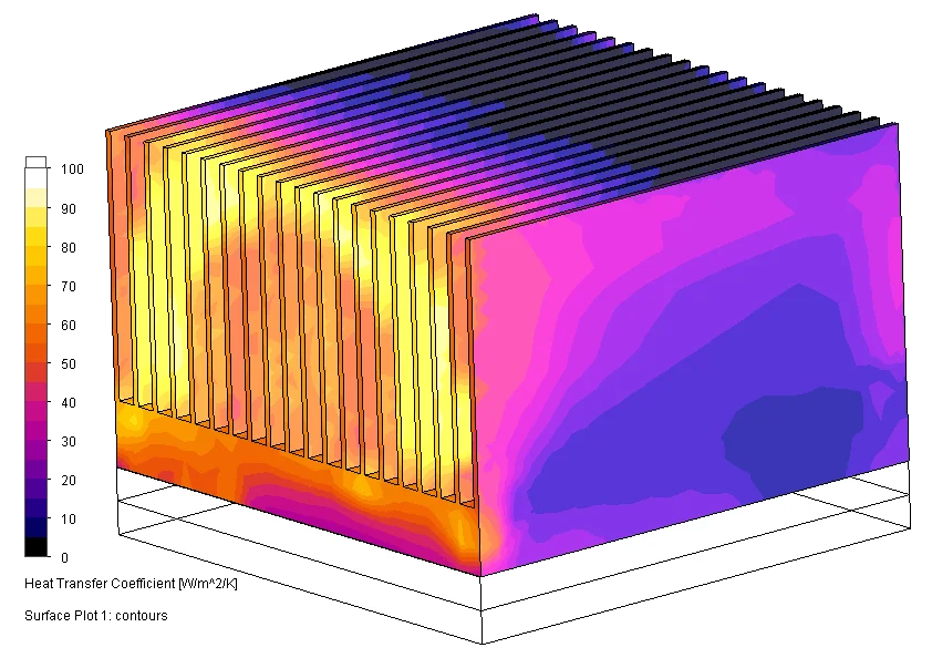
Image 3: Heat Transfer Coefficients [W/m2K] on a Heat Sink in a Forced Convection electronics enclosure with inlet fans.

In the next example, a simple test board with four chips is oriented vertically to gravity to allow more buoyant hot air to rise in a free convection problem. Image 4 shows a comparison of the heat transfer coefficient from the post-solution variation calculated by Flow Simulation on the left and the overall averaged 5.575 W/m²K applied as a known BC value a priori to all surfaces of the board in the Simulation Professional. The temperatures in Image 5 show that the distribution of temperatures for the Simulation Professional solution are much more uniform than the more realistic Flow Simulation results. The temperature of the chip in the upper left corner is different in the Flow Simulation result because it demonstrates how the hot air rising from the chip below causes it to become hotter than the Simulation Professional solution suggests; this is a direct correlation of the differing approaches for how convection is handled by the two different packages. Also notice that the legends show the values from ambient temperature of 20°C up to maximum calculated temperature, and notice how the Simulation Professional result is much lower than the Flow Simulation solution. Hypothetically if we were to theorize that both solutions are incorrect, I’d still prefer to err on the more conservative, higher temperature side. [Note that the value of 5.575 is on the lower side of free convection estimates for air typically ranging between 5 and 25 W/m²K. A value of 3.835 instead would have had it match the max temperature from Flow Simulation.

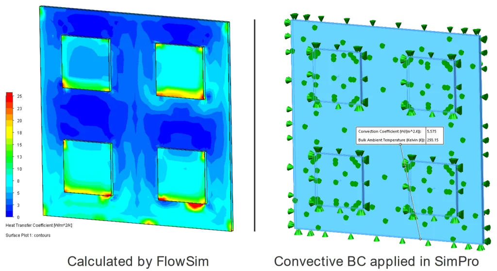
Image 4: On the left, Heat Transfer Coefficients [W/m²K] calculated for an external free convection problem solved by Flow Simulation, and on the right, a convection coefficient of 5.575 W/m²K applied as a BC on all external surfaces in Simulation Professional.

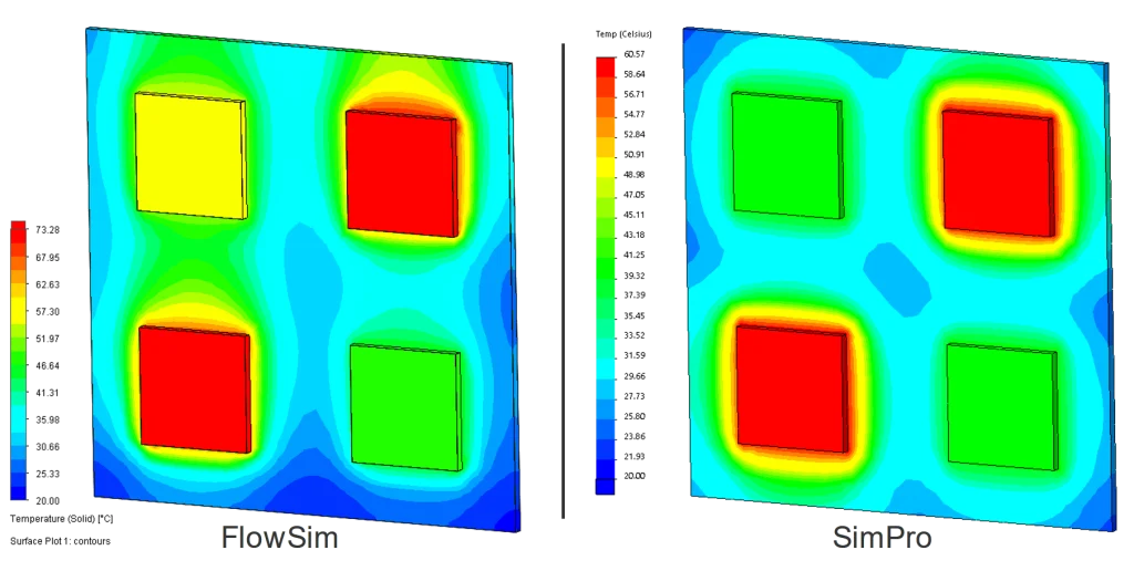
Image 5: Heat Transfer Coefficients [W/m2K] on a Heat Sink in a Forced Convection electronics enclosure with inlet fans

You might think that Radiation is not all important except when temperatures get really hot but you’d be mistaken, because it is one of the key cooling methods for a heat sink, for example, and if you don’t include it at even mild temperatures then it might be that little difference preventing the model from physical test results within a certain percentage. Thermal radiation is carried out in electromagnetic waves by photons for all bodies above absolute zero, 0 Kelvin, such that very hot objects like a molten rock glow red-hot in the visible spectrum.

When it comes to Radiation heat transfer, the capabilities of both Simulation Professional and Flow Simulation are the same at face value, but in practical usage is carried out differently; both are capable of doing solar/ambient radiation as well as body-to-body radiation. What ratio of thermal radiation an object “sees” (i.e. view factor) at its surface depends solely on geometry; think of sitting behind a tree in the shade during the daytime as opposed to out in front where the sun is shining. The way that Simulation Professional solves for the radiation view factor is by doing the calculation upfront before solving for temperatures. It entails a massive geometry problem of the contribution of each outwardly facing element face to every other element face participating in radiation; so because of this it is recommended to have a fairly coarse mesh in Simulation Professional that includes radiation, otherwise you could wait for a long time for the view factor calculation itself to complete, see Image 6. For the same model and mesh in Simulation Professional, it takes only 5 seconds to solve a problem with convection cooling, but when surface-to-surface radiation is included, the solution time took 147 minutes total with the view factor calculation taking about 70 minutes of that time; that is an increase of over 1750x in total time where view factor calculation uses 48% of that time. [Note that once the view factor calculation is performed, as long as mesh doesn’t change then it doesn’t need to be run again, for example if you want to test out a different power input.]

Whereas the Flow Simulation solver handles radiation, including the view factor calculation, simply by including it as part of the normal iterative solver. It seems that it does take a little bit longer to solve a model that includes radiation, but it is not a significant amount of time; the most that you see is a message at the bottom of the screen between each iteration for a few seconds that reads “Refining rays” while it updates, see Image 7.

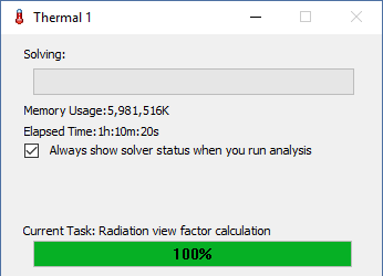
Image 6: Simulation Professional radiation view factor calculation dialog box.

Image 7: Flow Simulation solver updating radiation calculation message “Refining rays” at the bottom of the solver monitoring window.

The results for a conjugate heat transfer test “Lamp with reflector” model are shown in Image 8, where all three heat transfer modes were used in the solution. The time to solve the model in Simulation Professional with 85,564 elements was 2h27m22s, and for Flow Simulation with 82,703 solid cells (and 346,579 total cells including 263,876 fluid and fluid contacting solid cells) was 9m17s. With the size of the mesh being roughly equivalent, the Simulation Professional solution took nearly 16x longer to solve. The difference in time for solving a sample problem in Flow Simulation including radiation versus without was 1m48s longer, representing only a 24% increase.

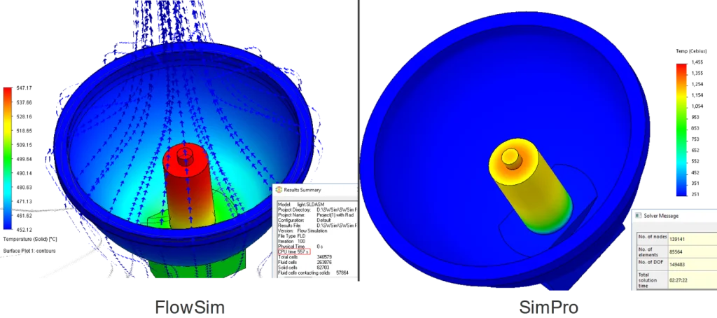
Image 8: Comparison of results for the test “Lamp with reflector” model solved as a conjugate heat transfer simulation including conduction, convection and radiation.

And finally one last example problem, this time only for Flow Simulation for a conjugate heat transfer problem on a PCB including free convection, conduction and radiation. The additional item that was considered in this problem was Ohmic (or Joule) heating in the copper traces where either a voltage potential or current can be introduced to electrical resistant materials, such as copper, to calculate amount of heat power dissipated in the circuit. This capability is available in Flow Simulation as an add-on Electronics Cooling package. Image 9 shows the radiant flux leaving from the hot components, and Image 10 shows a Flux Plot, which is new for the 2019 release, with radiation being the largest contributor (54%) to the cooling. According to the associated pie chart, about 30% goes to the surrounding fluid, due to both conducting and free convection to the air, and the remaining 16% to the sum of other much smaller individual fluxes that were filtered out of the plot.

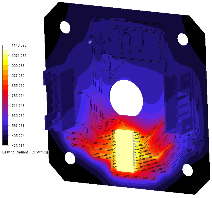
Image 9: Leaving Radiant Flux plot on a Stepper Motor Driver PCB model with copper traces.

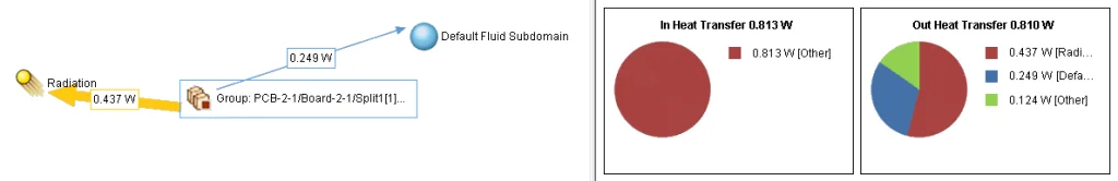
Image 10: Flux plot of heat leaving the PCB due to radiation and conduction and convection to the surrounding air fluid; a pie chart shows that radiation accounts for more than 50% of the heat transfer out.

Don’t forget to check back for the final part in the Flow Simulation’s Thermal Analysis Capabilities series on the SOLIDWORKS Tech Blog! Incase you missed it, take a look back on Part 1!

Bio
Twitter
LinkedIn
Latest Posts

Joe Galliera

Senior Simulation Technical Manager , East area at DS SOLIDWORKS

Joe Galliera has been with SOLIDWORKS since 2002. Previously he worked in the aerospace industry primarily focusing on computational methods. He geeks out on computational fluid dynamics (CFD) and nonlinear analysis.