The World is Nonlinear: Solving Buckling and Postbuckling Analysis of a Reinforced Panel

To me, the phrase ‘the world is nonlinear’ sums up why designers need access to powerful, yet easy to use simulation tools. Simply put ‘the world is nonlinear’ means that the response of a system is disproportional to the inputs. For structural simulation, this means that the components or assembly deformations are not proportional to the increase in loads. Many designers think that to be nonlinear, the loading has to be extreme. This is not the case, for many thin structures, the loads can be quite moderate while still exhibiting large deformations, such as when a system buckles. I have been lucky enough to be an intern at SIMULIA and decided to use their newest solution on the 3DEXPERIENCE platform, Structural Performance Engineer, to investigate both the prediction of buckling and the behavior of structure after it has buckled.

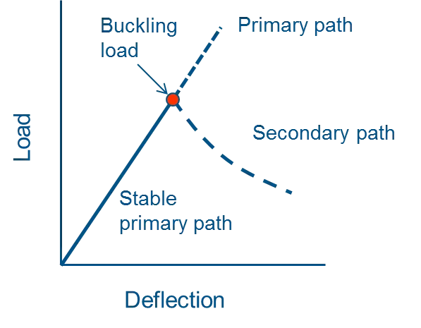
Buckling is a critical failure mode of structural components. It occurs when a structure loses its load-carrying capacity under compressive loading. The buckling load may be significantly lower than the ultimate stress needed to cause material yielding. This is why it is important to analyze buckling in safety-critical structures. When buckling occurs, the primary equilibrium path i.e. the load-displacement path experiences a bifurcation as shown in Figure 1. Beyond the bifurcation point is the secondary equilibrium path where the response of the structure may be highly nonlinear. This is the postbuckling regime.

Linear buckling analyses can provide some basic information about the buckling load. However, the collapse load of some structures is much higher than the buckling load predicted by a linear buckling (eigenvalue) analysis. In other cases, a structure will regain some of its load-carrying capacity after it buckles. In both of these cases, it is necessary to perform a nonlinear buckling analysis that includes postbuckling.

One complication that arises when performing nonlinear buckling analyses is that general static solvers which use the Newton-Raphson method fail to provide information about the postbuckling response of a structure due to the instability at the bifurcation point. This is particularly detrimental for snap-through buckling problems where a structure may have more than one stable load-carrying configuration. The high accelerations and inertial effects necessitate the need for a dynamic solver that accounts for the mass and inertia of the structure. Here, we explore how implicit dynamics in 3DEXPERIENCE can be used to model the nonlinear buckling and postbuckling response of a structure.

One example of a structure that may experience buckling is an aircraft fuselage panel. These panels consist of a thin skin reinforced with stringers in the longitudinal direction to improve their load-carrying capacity. Frames may also be added to improve stiffness in the circumferential direction but will be left out of this analysis for simplicity. The panel under consideration is shown in Figure 2.

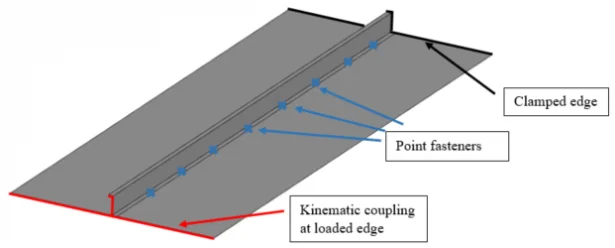
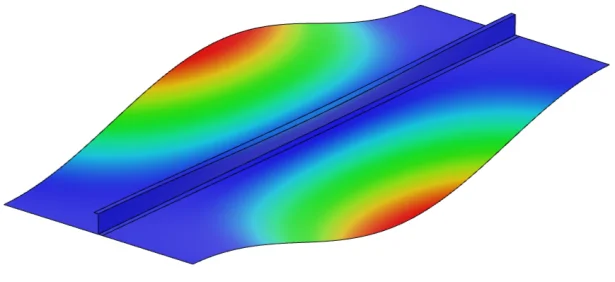
The panel consists of a thin rectangular skin of thickness 2 mm, length 600 mm, and width 220 mm. The skin is reinforced with a Z-beam stringer of thickness 1.6 mm, web height 25 mm, and flange width 20 mm. Since the thicknesses of the skin and stringer are very small compared to their other dimensions, the structure is modeled using S8R shell elements. Aluminum (Image = 70 GPa, Image = 0.3) with elastic-plastic material behavior is used for both parts. The stringer is fastened to the skin using point fasteners and kinematic coupling is defined at one edge of the panel such that the edges of the skin and stringer are coupled to a reference point. This reference point will be used to introduce force and displacement loading. The opposite edge of the panel is fully clamped. First, a linear buckling analysis is performed with a compressive load of 20 kN applied at the reference point on the loaded edge. The results indicate that the skin buckling load is approximately 18 kN. The buckled shape of the panel is shown in Figure 3.

For reinforced panels, the skin buckling load is typically much lower than the collapse load of the entire structure. Therefore, it is necessary to perform a complete nonlinear buckling analysis that includes postbuckling. In more complex simulations, a geometric imperfection based on the first few buckling modes could be introduced into the geometry prior to the postbuckling analysis. Alternatively, a loading imperfection could be introduced. It is well known that ‘imperfect’ structures have much lower buckling loads compared to ‘perfect’ structures. For the present analysis however, an imperfection is not introduced, as the goal is to demonstrate the robustness of the implicit dynamics solver.

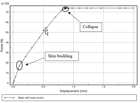
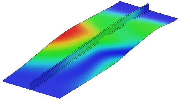
For comparison, the analysis is also performed using the static solver with stabilization to reduce inertial effects. In the static analysis, a compressive load of 100 kN is applied to the loaded edge. The load-displacement behavior obtained is shown in Figure 4. We can see that the skin buckles at a load of 17.68 kN as indicated by the slight kink in the response but the structure collapses at a much higher load i.e. approximately 74 kN. The buckled shape of the panel and the displacement magnitude contour is shown in Figure 5.

The static solver fails to provide a solution beyond a displacement of 2.0 mm. Therefore, we will perform a nonlinear buckling analysis using implicit dynamics with both load control and displacement control. For the load-controlled case, we apply a compressive load of 100 kN to the reference point on the loaded edge (similar to the static and eigenvalue analyses). For the displacement-controlled case, we apply a compressive displacement of 150 mm to the reference point. The force-displacement responses from both cases are shown in Figure 6.

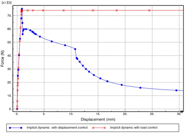
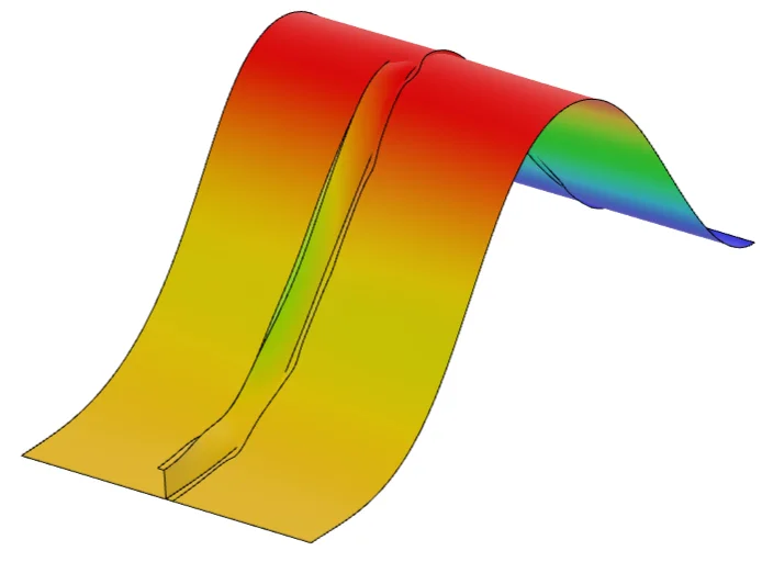
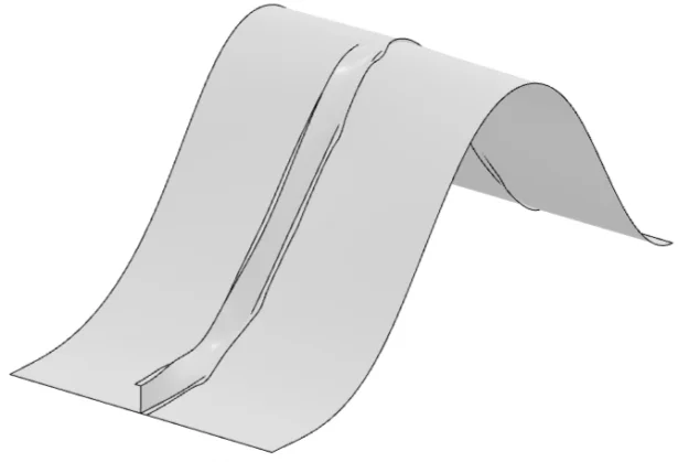
Using implicit dynamics, we can see that a postbuckling solution can easily be obtained. In this case, the solver does not face any issues producing a solution beyond the structures collapse load since we are taking into account the mass (inertia) of the panel and using it to solve the complete equations of motion in the time domain. As a result, the panel is able to sustain deformation well beyond the collapse load. The load-controlled case was manually terminated after the panel displacement reached 150 mm and the displacement-controlled case successfully provided a solution up to 150 mm. However, we can see that the panel does not regain any of its structural stiffness in the postbuckling regime. This is important for structural engineers who may want to investigate how the panel behaves after buckling, and is a particularly useful tool for snap-through type buckling problems, where a structure can have some stiffness beyond the buckling point. In this case, we can see that the panel continues to deform without any increase in the load. The final buckled shape is shown in Figure 7 and the displacement contours are shown in Figure 8.

For more information on Structural Performance Engineer, click here.